Predicting Bitcoin Price Direction Using Machine Learning
A Data-Driven Approach to Forecasting Cryptocurrency Trends
Introduction
Bitcoin, since its inception in 2009, has evolved from a niche digital currency to a significant player in global financial markets. Its volatility and unique nature have attracted not only traders but also researchers who aim to predict its price movements. However, most of the research in this area has been conducted post-2018, leaving room for exploration and innovation. In this study, I ventured into the complex world of Bitcoin price prediction, employing various machine learning methods to determine the direction of its price movements. This post outlines my approach, the unique aspects of my study, and the results that set it apart from existing literature.
What makes this study stand out is twofold: the data and variables used, and the comparative analysis of different machine learning methods. Unlike previous studies that often relied on a limited set of variables, I incorporated a wide range of predictors, including macro-economic and political factors, cryptocurrency-specific metrics, investor attention, day anomalies, and parallel market indicators. This comprehensive dataset, sourced from platforms like Quandl, Wikipedia, Yahoo Finance, and Investing, is detailed in Table 1 below.
Table 1. Input Variables and Their Sources
| Variable | Source |
|---|---|
| Daily economic policy uncertainty index (US) | EPU indices |
| Daily economic policy uncertainty index (UK) | EPU indices |
| Hash Rate | Quandl |
| Difficulty | Quandl |
| Estimated Transaction Value | Quandl |
| Total Transaction Fees | Quandl |
| my wallet number of transactions per day | Quandl |
| my wallet transaction volume | Quandl |
| average block size | Quandl |
| API Blockchain size | Quandl |
| Cost per transaction | Quandl |
| Cost % of transaction volume | Quandl |
| total output volume | Quandl |
| number of transactions per block | Quandl |
| Number of unique bitcoin addresses used | Quandl |
| Number of transactions excluding popular addresses | Quandl |
| Total transaction fee USD | Quandl |
| Number of transactions | Quandl |
| Total Bitcoin | Quandl |
| Wikipedia trend | Wikipedia |
| Day | Calculated |
| Type of Day (Weekday/Weekend) | Calculated |
| Lag 1 | Calculated |
| Lag 2 | Calculated |
| Bitcoin Price | coinmarketcap |
| Market capitalization | coinmarketcap |
| S&P 500 | Yahoo Finance |
| VIX | Yahoo Finance |
| Gold price | Investing |
Methodology
Given the complexity of predicting Bitcoin's price direction, I employed several machine learning models, including Lasso, Ridge, Elastic Net, Random Forest, and Support Vector Machine (SVM). Each model was chosen for its ability to handle the high-dimensional dataset effectively. For instance, Lasso, Ridge, and Elastic Net are well-suited for models with many predictors, while Random Forest offers flexibility in capturing both additive and interaction effects. The data preparation and analysis were conducted using Python, with all variables (except binary ones) normalized to have a mean of zero and a variance of one. Additionally, the variables were shifted by one day to measure their impact on the next day's return.
Data Splitting Strategy
When working with time series data, it's crucial to maintain the temporal order of observations. According to Machine Learning Mastery, there are three primary methods for splitting time series data into training and test sets:
- Train-Test Split: This method respects the temporal order and is ideal when a large dataset is available.
- Multiple Train-Test Splits: This approach also respects temporal order and allows for multiple evaluations.
- Walk-Forward Validation: Here, the model is updated with each new time step.
Given that my dataset was sizable, I opted for the Train-Test Split method, using the first three years of data for training and the last year for testing. This approach aligns with the method used in Section 4.6.3 of An Introduction to Statistical Learning (ISLR) when analyzing stock market data.
Results and Analysis
Given the 28 predictors in the dataset, models capable of handling high-dimensional data, such as Lasso, Ridge, Elastic Net, and Random Forest, were considered strong candidates for this analysis. However, I also explored and compared the performance of other methods to ensure a comprehensive evaluation.
All variables, except the binary ones, were normalized to have a mean of zero and a standard deviation of one. Additionally, the variables were shifted by one day to assess their impact on the following day's returns.
Table 2 presents the confusion matrices and accuracy rates of the models, ranked by their accuracy.
Table 2. Performance of the models
| Ridge | Accuracy | ||||
|---|---|---|---|---|---|
| Prediction/Output | Down | Up | 0.6066 | ||
| Down | 19 | 9 | |||
| Up | 135 | 203 | |||
| Lasso | Accuracy | ||||
| Prediction/Output | Down | Up | 0.6011 | ||
| Down | 14 | 6 | |||
| Up | 140 | 206 | |||
| Elastic net | Accuracy | ||||
| Prediction/Output | Down | Up | 0.6011 | ||
| Down | 13 | 5 | |||
| Up | 141 | 207 | |||
| OLS Post Lasso | Accuracy | ||||
| Prediction/Output | Down | Up | 0.5902 | ||
| Down | 10 | 6 | |||
| Up | 144 | 206 | |||
| Logit Post Lasso | Accuracy | ||||
| Prediction/Output | Down | Up | 0.5847 | ||
| Down | 14 | 12 | |||
| Up | 140 | 200 | |||
| OLS | Accuracy | ||||
| Prediction/Output | Down | Up | 0.5847 | ||
| Down | 16 | 14 | |||
| Up | 138 | 198 | |||
| LDA | Accuracy | ||||
| Prediction/Output | Down | Up | 0.582 | ||
| Down | 44 | 43 | |||
| Up | 110 | 169 | |||
| Logit | Accuracy | ||||
| Prediction/Output | Down | Up | 0.5792 | ||
| Down | 45 | 45 | |||
| Up | 109 | 167 | |||
| Ridge with cross-validation | Accuracy | ||||
| Prediction/Output | Down | Up | 0.5792 | ||
| Down | 0 | 0 | |||
| Up | 154 | 212 | |||
| OLS Backward selection model | Accuracy | ||||
| Prediction/Output | Down | Up | 0.5683 | ||
| Down | 51 | 55 | |||
| Up | 103 | 157 | |||
| QDA | Accuracy | ||||
| Prediction/Output | Down | Up | 0.5656 | ||
| Down | 12 | 17 | |||
| Up | 142 | 195 | |||
| SVM | Accuracy | ||||
| Prediction/Output | Down | Up | 0.5601 | ||
| Down | 25 | 32 | |||
| Up | 129 | 180 | |||
| GAM 2 Model (smoothing splines with degree of freedom of 10) | Accuracy | ||||
| Prediction/Output | Down | Up | 0.5418 | ||
| Down | 22 | 33 | |||
| Up | 132 | 179 | |||
| GAM 3 Model (Logit allowing for nonlinearity and lasso regularized) | Accuracy | ||||
| Prediction/Output | Down | Up | 0.535 | ||
| Down | 74 | 90 | |||
| Up | 80 | 122 | |||
| Random Forest | Accuracy | ||||
| Prediction/Output | Down | Up | 0.5191 | ||
| Down | 49 | 71 | |||
| Up | 105 | 141 | |||
| Bagging | Accuracy | ||||
| Prediction/Output | Down | Up | 0.459 | ||
| Down | 95 | 139 | |||
| Up | 59 | 73 | |||
| GAM 1 Model (smoothing splines with degree of freedom of 4) | Accuracy | ||||
| Prediction/Output | Down | Up | 0.4536 | ||
| Down | 102 | 148 | |||
| Up | 52 | 64 | |||
| Tree | Accuracy | ||||
| Prediction/Output | Down | Up | 0.4208 | ||
| Down | 154 | 212 | |||
| Up | 0 | 0 | |||
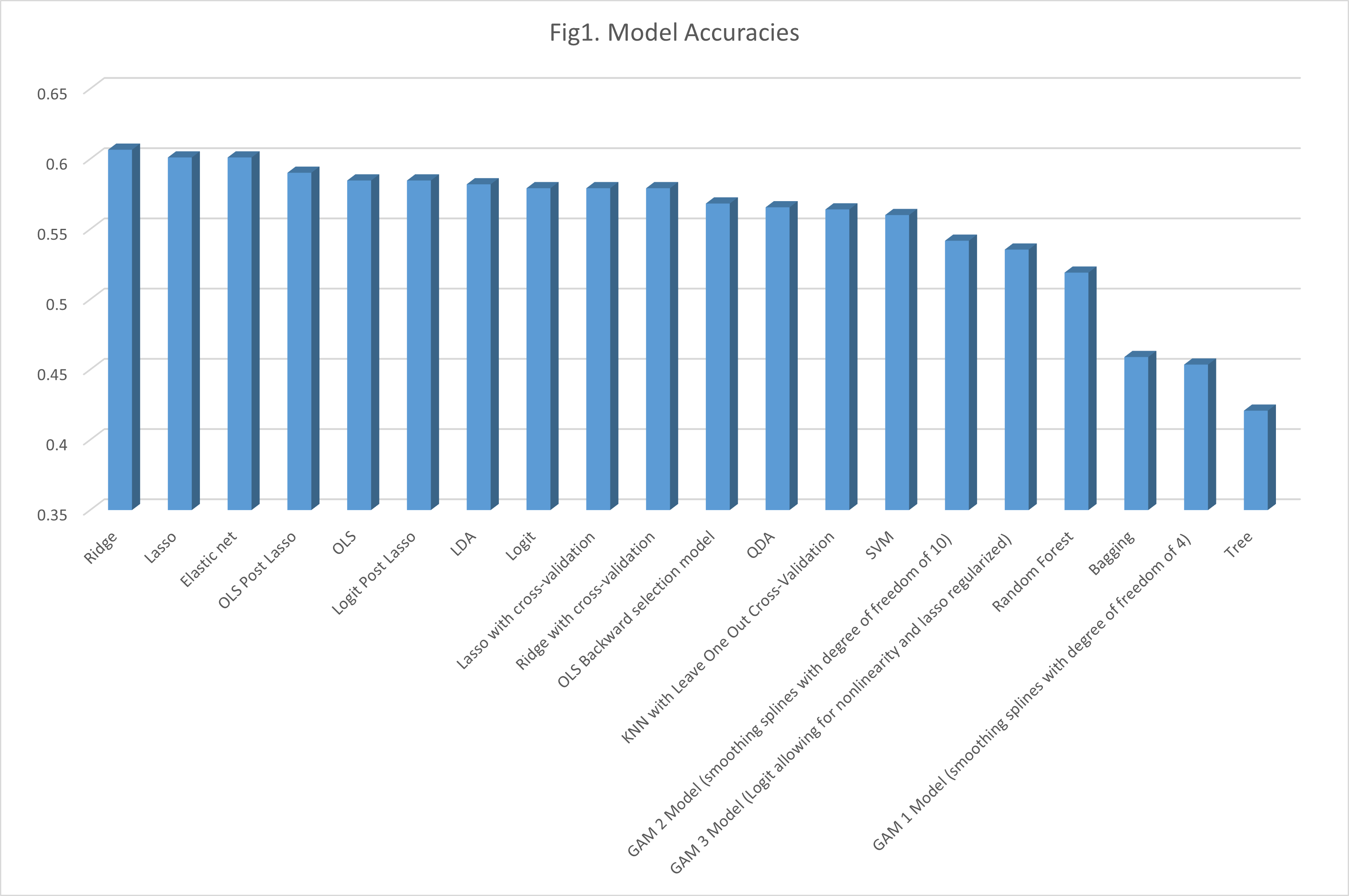
Table 2 highlights that models such as Lasso, Ridge, Elastic Net, OLS post-Lasso, and Logit post-Lasso demonstrate strong performance. Despite various adjustments in the Random Forest and SVM models, a simple OLS model emerged as the top performer.
Although the OLS model achieves an accuracy rate of 61%, this figure is only marginally better than the naïve models. Specifically, a naïve model predicting a down movement every day in the test sample achieves a correctness rate of 42.08%, while one predicting an up movement every day achieves 57.92%. Consequently, the 61% accuracy rate of the OLS model does not offer a significant advantage over the naïve model, supporting the efficient market hypothesis. This suggests that past information is already reflected in the prices, which follow a martingale process.
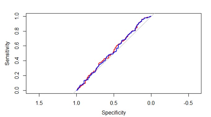
Figure 1 illustrates the ROC curves for the top two models. The ROC curve for the Ridge model (shown in red) and the Lasso model (shown in blue) both closely align with the 45-degree diagonal line, indicating that even the best models perform similarly. Other models exhibit comparable ROC curves, and if included, they would overlap with those depicted.
Figure 1. ROC curve